More Information

Submitted: 19 December 2019 | Approved: 10 February 2020 | Published: 11 February 2020

How to cite this article: Noori NM, Qasim OS. Improving cancer diseases classification using a hybrid filter and wrapper feature subset selection. Ann Proteom Bioinform. 2020; 4: 006-011.

DOI: 10.29328/journal.apb.1001010

Copyright License: © 2020 Noori NM, et al. This is an open access article distributed under the Creative Commons Attribution License, which permits unrestricted use, distribution, and reproduction in any medium, provided the original work is properly cited.

Keywords: Feature selection; Gray wolf optimization; Classification; Mutual information

 FullText PDF

Improving cancer diseases classification using a hybrid filter and wrapper feature subset selection

Noor Muhammed Noori* and Omar Saber Qasim

Department of Mathematics, University of Mosul, Mosul, Iraq

*Address for Correspondence: Noor Muhammed Noori, Department of Mathematics, University of Mosul, Mosul, Iraq, Tel: +964 7715381243; Email: NoorMuhammedNoori@uomosul.edu.iq

In the classification of cancer data sets, we note that they contain a number of additional features that influence the classification accuracy. There are many evolutionary algorithms that are used to define the feature and reduce dimensional patterns such as the gray wolf algorithm (GWO) after converting it from a continuous space to a discrete space. In this paper, a method of feature selection was proposed through two consecutive stages in the first stage, the fuzzy mutual information (FMI) technique is used to determine the most important feature selection of diseases dataset through a fuzzy model that was built based on the data size. In the second stage, the binary gray wolf optimization (BGWO) algorithm is used to determine a specific number of features affecting the process of classification, which came from the first stage. The proposed algorithm, FMI_BGWO, describes efficiency and effectiveness by obtaining a higher classification accuracy and a small number of selected genes compared to other competitor algorithms.

Mutual information (MI) is one of the filtering methods, which is calculated between two random variables using entropy. Entropy measures an average random variable the amount of information required to describe the random variable [1].

Gray wolf optimization (GWO) is a swarm intelligent technique developed by Mirjalili, et al. [2]. The hunting techniques and the social hierarchy of wolves are mathematically modeled in order to develop GWO and perform optimization. The GWO algorithm is tested with the standard test functions that indicate that it has superior exploration and exploitation characteristics than other swarm intelligence techniques [3]. Scientists have developed the basic algorithm GWO by converting the search algorithm from a continuous search space to a discrete search space. This modified algorithm is called a binary gray wolf optimization(BGWO) algorithm, which works in binary search areas and uses binary values ​​equal to 0 or 1 [3,4].

Feature subset selection method is a procedure to reduce the number of unnecessary feature from the original feature set [5,6]. This method is used when we have a large number of features in a dataset, where the method of determining the feature to take a number of features necessary. The feature selection can be applied in several areas and is intended to improve the accuracy of the classification. Two basic methods are used in selecting the feature: filtering approaches, wrapper approaches.

In this study, a new FMI_BGWO algorithm is suggested to determine the best-feature selection. Our proposed algorithm can efficiently achievement the powerful points of both FMI and BGWO algorithms in finding the most important feature. The experimental results show the excellent performance of the proposed algorithm when the number of feature is high, and the sample size is low.

The remains of this paper are organized as follows. The GWO is presented in Section 2. In Sections 3 and 4, a brief description of feature selection and MI respectively. In Section 5, the proposed algorithm is explained. Section 6 covers the obtained results and their discussion. Finally, the most important general conclusions are mentioned, in section 7.

Grey Wolf Optimization (GWO)

The gray wolf (Canis lupus) is part of the Canidae family. Gray wolves are types with a very rigorous social dominant hierarchy of leadership. Males and females in the pack are leaders, and they are called alpha [2]. Alpha wolf is also known as the dominant wolf because all its orders must be followed by all wolves in the pack. Only alpha wolves are allowed to mate in the pack. This means that the order of the pack and its regularity is more important than its strength. Beta is the second level in the hierarchy of gray wolves.

Beta are wolves that help alpha wolves make decisions or other things about the pack. The wolf beta is the best candidate to be alpha in the case if one of the wolves of alpha becomes too big or in the case of the death of someone in command.

Omega is less gray wolves. The omega wolf always offers all the other dominant wolves on it. Omega acts as a scapegoat. The last wolves allowed to eat are omega. We may apparently notice that omega is not an important member of the group, but in fact, if omega is lost, the entire pack will face problems and internal fighting.

Delta is the fourth class in the pack. Delta wolves control omega, but they must undergo alpha and beta orders. Delta shall be responsible for guards, scouts, hunters, elders, and patients and each has its own specific responsibility [7].

Mathematical modelling

The first best solution in GWO is alpha (α), the second-best solution is beta (β), and the third-best solution is Delta (δ). While the rest of the solutions are Omega (ω), which follows the rest of the first three solutions [8].

Encircling prey: Gray wolves surrounded prey while hunting. The following equations will represent a mathematical model about the surrounding behavior:

X ( t+1 )= X p ( t )  A D     (1) MathType@MTEF@5@5@+=feaaguart1ev2aaatCvAUfeBSjuyZL2yd9gzLbvyNv2CaerbuLwBLnhiov2DGi1BTfMBaeXatLxBI9gBaerbd9wDYLwzYbItLDharqqtubsr4rNCHbGeaGqk0Jf9crFfpeea0xh9v8qiW7rqqrFfpeea0xe9Lq=Jc9vqaqpepm0xbba9pwe9Q8fs0=yqaqpepae9pg0FirpepeKkFr0xfr=xfr=xb9adbaqaaeGaciGaaiaabeqaamaabaabaaGcbaWaaCbiaeaaqaaaaaaaaaWdbiaadIfaaSWdaeqabaWdbiabgkziUcaakmaabmaapaqaa8qacaqG0bGaey4kaSIaaGymaaGaayjkaiaawMcaaiabg2da98aadaWfGaqaa8qacaWGybWdamaaBaaaleaapeGaamiCaaWdaeqaaaqabeaapeGaeyOKH4kaaOWaaeWaa8aabaWdbiaadshaaiaawIcacaGLPaaacqGHsislcaGGGcWdamaaxacabaWdbiaadgeaaSWdaeqabaWdbiabgkziUcaakiabgwSix=aadaWfGaqaa8qacaWGebaal8aabeqaa8qacqGHsgIRaaGccaGGGcGaaeiiaiaabccacaqGGaGaaiikaiaaigdacaGGPaaaaa@57DB@

D =| C   X p ( t ) X ( t ) |    ( 2 ) MathType@MTEF@5@5@+=feaaguart1ev2aaatCvAUfeBSjuyZL2yd9gzLbvyNv2CaerbuLwBLnhiov2DGi1BTfMBaeXatLxBI9gBaerbd9wDYLwzYbItLDharqqtubsr4rNCHbGeaGqk0Jf9crFfpeea0xh9v8qiW7rqqrFfpeea0xe9Lq=Jc9vqaqpepm0xbba9pwe9Q8fs0=yqaqpepae9pg0FirpepeKkFr0xfr=xfr=xb9adbaqaaeGaciGaaiaabeqaamaabaabaaGcbaWaaCbiaeaaqaaaaaaaaaWdbiaadseaaSWdaeqabaWdbiabgkziUcaakiabg2da9maaemaapaqaamaaxacabaWdbiaadoeaaSWdaeqabaWdbiabgkziUcaakiabgwSixlaacckapaWaaCbiaeaapeGaamiwa8aadaWgaaWcbaWdbiaadchaa8aabeaaaeqabaWdbiabgkziUcaakmaabmaapaqaa8qacaWG0baacaGLOaGaayzkaaGaeyOeI0YdamaaxacabaWdbiaadIfaaSWdaeqabaWdbiabgkziUcaakmaabmaapaqaa8qacaWG0baacaGLOaGaayzkaaaacaGLhWUaayjcSdGaaeiiaiaabccacaqGGaGaaiiOamaabmaapaqaa8qacaaIYaaacaGLOaGaayzkaaaaaa@59B4@

where t is the iteration,   X p MathType@MTEF@5@5@+=feaaguart1ev2aaatCvAUfeBSjuyZL2yd9gzLbvyNv2CaerbuLwBLnhiov2DGi1BTfMBaeXatLxBI9gBaerbd9wDYLwzYbItLDharqqtubsr4rNCHbGeaGqk0Jf9crFfpeea0xh9v8qiW7rqqrFfpeea0xe9Lq=Jc9vqaqpepm0xbba9pwe9Q8fs0=yqaqpepae9pg0FirpepeKkFr0xfr=xfr=xb9adbaqaaeGaciGaaiaabeqaamaabaabaaGcbaGaaiiOamaaxacabaaeaaaaaaaaa8qacaWGybWdamaaBaaaleaapeGaamiCaaWdaeqaaaqabeaapeGaeyOKH4kaaaaa@3DB0@ is the prey position, X MathType@MTEF@5@5@+=feaaguart1ev2aaatCvAUfeBSjuyZL2yd9gzLbvyNv2CaerbuLwBLnhiov2DGi1BTfMBaeXatLxBI9gBaerbd9wDYLwzYbItLDharqqtubsr4rNCHbGeaGqk0Jf9crFfpeea0xh9v8qiW7rqqrFfpeea0xe9Lq=Jc9vqaqpepm0xbba9pwe9Q8fs0=yqaqpepae9pg0FirpepeKkFr0xfr=xfr=xb9adbaqaaeGaciGaaiaabeqaamaabaabaaGcbaWaaCbiaeaaqaaaaaaaaaWdbiaadIfaaSWdaeqabaWdbiabgkziUcaaaaa@3B57@ is the gray wolf position,

the MathType@MTEF@5@5@+=feaaguart1ev2aaatCvAUfeBSjuyZL2yd9gzLbvyNv2CaerbuLwBLnhiov2DGi1BTfMBaeXatLxBI9gBaerbd9wDYLwzYbItLDharqqtubsr4rNCHbGeaGqk0Jf9crFfpeea0xh9v8qiW7rqqrFfpeea0xe9Lq=Jc9vqaqpepm0xbba9pwe9Q8fs0=yqaqpepae9pg0FirpepeKkFr0xfr=xfr=xb9adbaqaaeGaciGaaiaabeqaamaabaabaaGcbaaeaaaaaaaaa8qacqGHflY1aaa@3A6F@ operator indicates vector entry wise multiplication.

Where A MathType@MTEF@5@5@+=feaaguart1ev2aaatCvAUfeBSjuyZL2yd9gzLbvyNv2CaerbuLwBLnhiov2DGi1BTfMBaeXatLxBI9gBaerbd9wDYLwzYbItLDharqqtubsr4rNCHbGeaGqk0Jf9crFfpeea0xh9v8qiW7rqqrFfpeea0xe9Lq=Jc9vqaqpepm0xbba9pwe9Q8fs0=yqaqpepae9pg0FirpepeKkFr0xfr=xfr=xb9adbaqaaeGaciGaaiaabeqaamaabaabaaGcbaWaaCbiaeaaqaaaaaaaaaWdbiaadgeaaSWdaeqabaWdbiabgkziUcaaaaa@3B40@ and C MathType@MTEF@5@5@+=feaaguart1ev2aaatCvAUfeBSjuyZL2yd9gzLbvyNv2CaerbuLwBLnhiov2DGi1BTfMBaeXatLxBI9gBaerbd9wDYLwzYbItLDharqqtubsr4rNCHbGeaGqk0Jf9crFfpeea0xh9v8qiW7rqqrFfpeea0xe9Lq=Jc9vqaqpepm0xbba9pwe9Q8fs0=yqaqpepae9pg0FirpepeKkFr0xfr=xfr=xb9adbaqaaeGaciGaaiaabeqaamaabaabaaGcbaWaaCbiaeaaqaaaaaaaaaWdbiaadoeaaSWdaeqabaWdbiabgkziUcaaaaa@3B42@ are coefficient vectors calculated as follows:

  A =2 a r 1 a    (3) MathType@MTEF@5@5@+=feaaguart1ev2aaatCvAUfeBSjuyZL2yd9gzLbvyNv2CaerbuLwBLnhiov2DGi1BTfMBaeXatLxBI9gBaerbd9wDYLwzYbItLDharqqtubsr4rNCHbGeaGqk0Jf9crFfpeea0xh9v8qiW7rqqrFfpeea0xe9Lq=Jc9vqaqpepm0xbba9pwe9Q8fs0=yqaqpepae9pg0FirpepeKkFr0xfr=xfr=xb9adbaqaaeGaciGaaiaabeqaamaabaabaaGcbaGaaiiOamaaxacabaaeaaaaaaaaa8qacaWGbbaal8aabeqaa8qacqGHsgIRaaGccqGH9aqpcaaIYaWdamaaxacabaWdbiaadggaaSWdaeqabaWdbiabgkziUcaakiabgwSix=aadaWfGaqaa8qacaWGYbWdamaaBaaaleaapeGaaGymaaWdaeqaaaqabeaapeGaeyOKH4kaaOGaeyOeI0IaamyyaiaacckacaqGGaGaaeiiaiaabccacaGGOaGaaG4maiaacMcaaaa@4F44@

C =2  r 2     (4) MathType@MTEF@5@5@+=feaaguart1ev2aaatCvAUfeBSjuyZL2yd9gzLbvyNv2CaerbuLwBLnhiov2DGi1BTfMBaeXatLxBI9gBaerbd9wDYLwzYbItLDharqqtubsr4rNCHbGeaGqk0Jf9crFfpeea0xh9v8qiW7rqqrFfpeea0xe9Lq=Jc9vqaqpepm0xbba9pwe9Q8fs0=yqaqpepae9pg0FirpepeKkFr0xfr=xfr=xb9adbaqaaeGaciGaaiaabeqaamaabaabaaGcbaWaaCbiaeaaqaaaaaaaaaWdbiaadoeaaSWdaeqabaWdbiabgkziUcaakiabg2da9iaaikdacaGGGcWdamaaxacabaWdbiaadkhapaWaaSbaaSqaa8qacaaIYaaapaqabaaabeqaa8qacqGHsgIRaaGccaqGGcGaaeiiaiaabccacaqGGaGaaiikaiaaisdacaGGPaaaaa@47C6@

where components of a MathType@MTEF@5@5@+=feaaguart1ev2aaatCvAUfeBSjuyZL2yd9gzLbvyNv2CaerbuLwBLnhiov2DGi1BTfMBaeXatLxBI9gBaerbd9wDYLwzYbItLDharqqtubsr4rNCHbGeaGqk0Jf9crFfpeea0xh9v8qiW7rqqrFfpeea0xe9Lq=Jc9vqaqpepm0xbba9pwe9Q8fs0=yqaqpepae9pg0FirpepeKkFr0xfr=xfr=xb9adbaqaaeGaciGaaiaabeqaamaabaabaaGcbaGabmyyayaalaaaaa@38FD@ are linearly decreased from 2 to 0 over the course of iterations and r1, r2, are random vectors in [0,1].

Hunting: Gray wolves have the ability to encircle prey and locate them. Hunting is performed by a complete pack based on, Information from the alpha, beta and delta wolves, so the updating for the wolves positions is as in the following equations:

X ( t+1 )= X 1 + X 2 + X 3 3      (5) MathType@MTEF@5@5@+=feaaguart1ev2aaatCvAUfeBSjuyZL2yd9gzLbvyNv2CaerbuLwBLnhiov2DGi1BTfMBaeXatLxBI9gBaerbd9wDYLwzYbItLDharqqtubsr4rNCHbGeaGqk0Jf9crFfpeea0xh9v8qiW7rqqrFfpeea0xe9Lq=Jc9vqaqpepm0xbba9pwe9Q8fs0=yqaqpepae9pg0FirpepeKkFr0xfr=xfr=xb9adbaqaaeGaciGaaiaabeqaamaabaabaaGcbaWaaCbiaeaaqaaaaaaaaaWdbiaadIfaaSWdaeqabaWdbiabgkziUcaakmaabmaapaqaa8qacaWG0bGaey4kaSIaaGymaaGaayjkaiaawMcaaiabg2da9maalaaapaqaamaaxacabaWdbiaadIfapaWaaSbaaSqaa8qacaaIXaaapaqabaaabeqaa8qacqGHsgIRaaGccqGHRaWkpaWaaCbiaeaapeGaamiwa8aadaWgaaWcbaWdbiaaikdaa8aabeaaaeqabaWdbiabgkziUcaakiabgUcaR8aadaWfGaqaa8qacaWGybWdamaaBaaaleaapeGaaG4maaWdaeqaaaqabeaapeGaeyOKH4kaaaGcpaqaa8qacaaIZaaaaiaacckacaqGGaGaaeiiaiaabccacaqGGaGaaiikaiaaiwdacaGGPaaaaa@5622@

X 1 =| X α A 1 · D α | ,  X 2 =| X β A 2 · D β | ,  X 3 =| X δ A 3 · D δ |     (6) MathType@MTEF@5@5@+=feaaguart1ev2aaatCvAUfeBSjuyZL2yd9gzLbvyNv2CaerbuLwBLnhiov2DGi1BTfMBaeXatLxBI9gBaerbd9wDYLwzYbItLDharqqtubsr4rNCHbGeaGqk0Jf9crFfpeea0xh9v8qiW7rqqrFfpeea0xe9Lq=Jc9vqaqpepm0xbba9pwe9Q8fs0=yqaqpepae9pg0FirpepeKkFr0xfr=xfr=xb9adbaqaaeGaciGaaiaabeqaamaabaabaaGcbaWaaCbiaeaaqaaaaaaaaaWdbiaadIfapaWaaSbaaSqaa8qacaaIXaaapaqabaaabeqaa8qacqGHsgIRaaGccqGH9aqpdaabdaWdaeaadaWfGaqaa8qacaWGybWdamaaBaaaleaapeGaeqySdegapaqabaaabeqaa8qacqGHsgIRaaGccqGHsislpaWaaCbiaeaapeGaamyqa8aadaWgaaWcbaWdbiaaigdaa8aabeaaaeqabaWdbiabgkziUcaakiabl+y6N9aadaWfGaqaa8qacaWGebWdamaaBaaaleaapeGaeqySdegapaqabaaabeqaa8qacqGHsgIRaaaakiaawEa7caGLiWoacaGGGcGaaiilaiaacckapaWaaCbiaeaapeGaamiwa8aadaWgaaWcbaWdbiaaikdaa8aabeaaaeqabaWdbiabgkziUcaakiabg2da9maaemaapaqaamaaxacabaWdbiaadIfapaWaaSbaaSqaa8qacqaHYoGya8aabeaaaeqabaWdbiabgkziUcaakiabgkHiT8aadaWfGaqaa8qacaWGbbWdamaaBaaaleaapeGaaGOmaaWdaeqaaaqabeaapeGaeyOKH4kaaOGaeS4JPF2damaaxacabaWdbiaadseapaWaaSbaaSqaa8qacqaHYoGya8aabeaaaeqabaWdbiabgkziUcaaaOGaay5bSlaawIa7aiaacckacaGGSaGaaiiOa8aadaWfGaqaa8qacaWGybWdamaaBaaaleaapeGaaG4maaWdaeqaaaqabeaapeGaeyOKH4kaaOGaeyypa0ZaaqWaa8aabaWaaCbiaeaapeGaamiwa8aadaWgaaWcbaWdbiabes7aKbWdaeqaaaqabeaapeGaeyOKH4kaaOGaeyOeI0YdamaaxacabaWdbiaadgeapaWaaSbaaSqaa8qacaaIZaaapaqabaaabeqaa8qacqGHsgIRaaGccqWIpM+zpaWaaCbiaeaapeGaamira8aadaWgaaWcbaWdbiabes7aKbWdaeqaaaqabeaapeGaeyOKH4kaaaGccaGLhWUaayjcSdGaaeiOaiaabccacaqGGaGaaeiiaiaabccacaGGOaGaaGOnaiaacMcaaaa@9342@

D α =| C 1 · X α X | ,  D β =| C 2 · X β X | ,  D δ =| C 3 · X δ X |     (7) MathType@MTEF@5@5@+=feaaguart1ev2aaatCvAUfeBSjuyZL2yd9gzLbvyNv2CaerbuLwBLnhiov2DGi1BTfMBaeXatLxBI9gBaerbd9wDYLwzYbItLDharqqtubsr4rNCHbGeaGqk0Jf9crFfpeea0xh9v8qiW7rqqrFfpeea0xe9Lq=Jc9vqaqpepm0xbba9pwe9Q8fs0=yqaqpepae9pg0FirpepeKkFr0xfr=xfr=xb9adbaqaaeGaciGaaiaabeqaamaabaabaaGcbaWaaCbiaeaaqaaaaaaaaaWdbiaadseapaWaaSbaaSqaa8qacqaHXoqya8aabeaaaeqabaWdbiabgkziUcaakiabg2da9maaemaapaqaamaaxacabaWdbiaadoeapaWaaSbaaSqaa8qacaaIXaaapaqabaaabeqaa8qacqGHsgIRaaGccWaMaU4JPF2damaaxacabaWdbiaadIfapaWaaSbaaSqaa8qacqaHXoqya8aabeaaaeqabaWdbiabgkziUcaakiabgkHiT8aadaWfGaqaa8qacaWGybaal8aabeqaa8qacqGHsgIRaaaakiaawEa7caGLiWoacaqGGcGaaiilaiaabckapaWaaCbiaeaapeGaamira8aadaWgaaWcbaWdbiabek7aIbWdaeqaaaqabeaapeGaeyOKH4kaaOGaeyypa0ZaaqWaa8aabaWaaCbiaeaapeGaam4qa8aadaWgaaWcbaWdbiaaikdaa8aabeaaaeqabaWdbiabgkziUcaakiabl+y6N9aadaWfGaqaa8qacaWGybWdamaaBaaaleaapeGaeqOSdigapaqabaaabeqaa8qacqGHsgIRaaGccqGHsislpaWaaCbiaeaapeGaamiwaaWcpaqabeaapeGaeyOKH4kaaaGccaGLhWUaayjcSdGaaeiOaiaacYcacaqGGcWdamaaxacabaWdbiaadseapaWaaSbaaSqaa8qacqaH0oaza8aabeaaaeqabaWdbiabgkziUcaakiabg2da9maaemaapaqaamaaxacabaWdbiaadoeapaWaaSbaaSqaa8qacaaIZaaapaqabaaabeqaa8qacqGHsgIRaaGccqWIpM+zpaWaaCbiaeaapeGaamiwa8aadaWgaaWcbaWdbiabes7aKbWdaeqaaaqabeaapeGaeyOKH4kaaOGaeyOeI0YdamaaxacabaWdbiaadIfaaSWdaeqabaWdbiabgkziUcaaaOGaay5bSlaawIa7aiaabccacaqGGaGaaeiiaiaabccacaqGGcGaaiikaiaaiEdacaGGPaaaaa@9171@

The updating of the parameter a MathType@MTEF@5@5@+=feaaguart1ev2aaatCvAUfeBSjuyZL2yd9gzLbvyNv2CaerbuLwBLnhiov2DGi1BTfMBaeXatLxBI9gBaerbd9wDYLwzYbItLDharqqtubsr4rNCHbGeaGqk0Jf9crFfpeea0xh9v8qiW7rqqrFfpeea0xe9Lq=Jc9vqaqpepm0xbba9pwe9Q8fs0=yqaqpepae9pg0FirpepeKkFr0xfr=xfr=xb9adbaqaaeGaciGaaiaabeqaamaabaabaaGcbaGabmyyayaalaaaaa@38FD@ through the following equation:

a =2t   2 Ma x iter       (8) MathType@MTEF@5@5@+=feaaguart1ev2aaatCvAUfeBSjuyZL2yd9gzLbvyNv2CaerbuLwBLnhiov2DGi1BTfMBaeXatLxBI9gBaerbd9wDYLwzYbItLDharqqtubsr4rNCHbGeaGqk0Jf9crFfpeea0xh9v8qiW7rqqrFfpeea0xe9Lq=Jc9vqaqpepm0xbba9pwe9Q8fs0=yqaqpepae9pg0FirpepeKkFr0xfr=xfr=xb9adbaqaaeGaciGaaiaabeqaamaabaabaaGcbaWaaCbiaeaaqaaaaaaaaaWdbiaadggaaSWdaeqabaWdbiabgkziUcaakiabg2da9iaaikdacqGHsislcaWG0bGaaeiiaiabgwSixlaabccadaWcaaWdaeaapeGaaGOmaaWdaeaapeGaamytaiaadggacaWG4bWdamaaBaaaleaapeGaamyAaiaadshacaWGLbGaamOCaaWdaeqaaaaak8qacaqGGaGaaeiiaiaabccacaqGGaGaaeiiaiaabckacaGGOaGaaGioaiaacMcaaaa@510A@

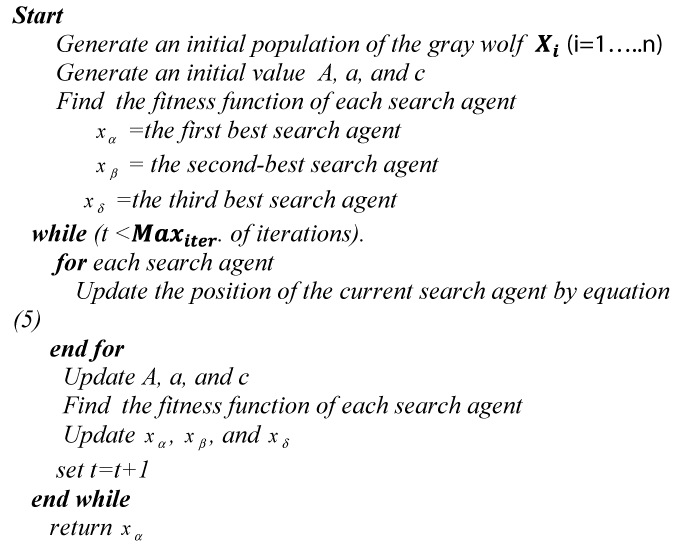
Where t is the iteration number and Maxiter is the total number of iteration allowed for the optimization [9]. The pseudo code of the GWO algorithm is displayed in figure 1.


Download Image

Figure 1: The pseudo code of the GWO algorithm.

Binary Gray Wolf Optimization (BGWO)

The positions of gray wolves constantly change in space to any point. Solutions are limited to binary values such as 0 or 1 in some special problems such as feature selection. In our research, we suggested feature selection through a binary GWO algorithm. Updating the equations of wolves are a function of the positions of three vectors is, Xa, Xβ and Xε which represents the best three solutions and which attracts each wolf towards it. At any given time, all solutions are at a corner of a hypercube and the solutions are grouped in binary form. Based on the basic GWO algorithm, the given wolf positions are updated, a binary restriction must be maintained according to equation (9).

The main update equation in the GWO algorithm is written as [3]:

X i t+1 =Crossover( X 1 , X 2 , X 3 )     (9) MathType@MTEF@5@5@+=feaaguart1ev2aaatCvAUfeBSjuyZL2yd9gzLbvyNv2CaerbuLwBLnhiov2DGi1BTfMBaeXatLxBI9gBaerbd9wDYLwzYbItLDharqqtubsr4rNCHbGeaGqk0Jf9crFfpeea0xh9v8qiW7rqqrFfpeea0xe9Lq=Jc9vqaqpepm0xbba9pwe9Q8fs0=yqaqpepae9pg0FirpepeKkFr0xfr=xfr=xb9adbaqaaeGaciGaaiaabeqaamaabaabaaGcbaaeaaaaaaaaa8qacaWGybWdamaaDaaaleaapeGaamyAaaWdaeaapeGaamiDaiabgUcaRiaaigdaaaGccqGH9aqpcaWGdbGaamOCaiaad+gacaWGZbGaam4Caiaad+gacaWG2bGaamyzaiaadkhadaqadaWdaeaapeGaamiwa8aadaWgaaWcbaWdbiaaigdaa8aabeaak8qacaGGSaGaamiwa8aadaWgaaWcbaWdbiaaikdaa8aabeaak8qacaGGSaGaamiwa8aadaWgaaWcbaWdbiaaiodaa8aabeaaaOWdbiaawIcacaGLPaaacaqGGaGaaeiiaiaabccacaqGGaGaaeiOaiaacIcacaaI5aGaaiykaaaa@556E@

Where (X1, X2, X3) they are binary vectors representing wolves in bGWO and crossover (a, b, c) are an appropriate intersection between solutions (a, b, c) and (X1, X2, X3), and the wolves calculate alpha, beta and delta in order using equations (10), (13) and (16).

X 1 d ={ 1 if ( X α d +bste p α d )1 0 other wise       (10) MathType@MTEF@5@5@+=feaaguart1ev2aaatCvAUfeBSjuyZL2yd9gzLbvyNv2CaerbuLwBLnhiov2DGi1BTfMBaeXatLxBI9gBaerbd9wDYLwzYbItLDharqqtubsr4rNCHbGeaGqk0Jf9crFfpeea0xh9v8qiW7rqqrFfpeea0xe9Lq=Jc9vqaqpepm0xbba9pwe9Q8fs0=yqaqpepae9pg0FirpepeKkFr0xfr=xfr=xb9adbaqaaeGaciGaaiaabeqaamaabaabaaGcbaaeaaaaaaaaa8qacaWGybWdamaaDaaaleaapeGaaGymaaWdaeaapeGaamizaaaakiabg2da9maaceaapaqaauaabeqaceaaaeaapeGaaGymaiaacckacaWGPbGaamOzaiaacckacaGGOaGaamiwa8aadaqhaaWcbaWdbiabeg7aHbWdaeaapeGaamizaaaakiabgUcaRiaadkgacaWGZbGaamiDaiaadwgacaWGWbWdamaaDaaaleaapeGaeqySdegapaqaa8qacaWGKbaaaOGaaiykaiabgwMiZkaaigdaa8aabaWdbiaaicdacaGGGcGaam4BaiaadshacaWGObGaamyzaiaadkhacaGGGcGaam4DaiaadMgacaWGZbGaamyzaiaacckaaaaacaGL7baacaqGGaGaaeiiaiaabccacaqGGaGaaeiOaiaacIcacaaIXaGaaGimaiaacMcaaaa@65D6@

Where bste p α d MathType@MTEF@5@5@+=feaaguart1ev2aaatCvAUfeBSjuyZL2yd9gzLbvyNv2CaerbuLwBLnhiov2DGi1BTfMBaeXatLxBI9gBaerbd9wDYLwzYbItLDharqqtubsr4rNCHbGeaGqk0Jf9crFfpeea0xh9v8qiW7rqqrFfpeea0xe9Lq=Jc9vqaqpepm0xbba9pwe9Q8fs0=yqaqpepae9pg0FirpepeKkFr0xfr=xfr=xb9adbaqaaeGaciGaaiaabeqaamaabaabaaGcbaaeaaaaaaaaa8qacaWGIbGaam4CaiaadshacaWGLbGaamiCa8aadaqhaaWcbaWdbiabeg7aHbWdaeaapeGaamizaaaaaaa@3FCF@ is a binary step in dimension d, X α d MathType@MTEF@5@5@+=feaaguart1ev2aaatCvAUfeBSjuyZL2yd9gzLbvyNv2CaerbuLwBLnhiov2DGi1BTfMBaeXatLxBI9gBaerbd9wDYLwzYbItLDharqqtubsr4rNCHbGeaGqk0Jf9crFfpeea0xh9v8qiW7rqqrFfpeea0xe9Lq=Jc9vqaqpepm0xbba9pwe9Q8fs0=yqaqpepae9pg0FirpepeKkFr0xfr=xfr=xb9adbaqaaeGaciGaaiaabeqaamaabaabaaGcbaaeaaaaaaaaa8qacaWGybWdamaaDaaaleaapeGaeqySdegapaqaa8qacaWGKbaaaaaa@3BF5@ is a vector representing the position of the alpha wolf in dimension d. bste p α d MathType@MTEF@5@5@+=feaaguart1ev2aaatCvAUfeBSjuyZL2yd9gzLbvyNv2CaerbuLwBLnhiov2DGi1BTfMBaeXatLxBI9gBaerbd9wDYLwzYbItLDharqqtubsr4rNCHbGeaGqk0Jf9crFfpeea0xh9v8qiW7rqqrFfpeea0xe9Lq=Jc9vqaqpepm0xbba9pwe9Q8fs0=yqaqpepae9pg0FirpepeKkFr0xfr=xfr=xb9adbaqaaeGaciGaaiaabeqaamaabaabaaGcbaaeaaaaaaaaa8qacaWGIbGaam4CaiaadshacaWGLbGaamiCa8aadaqhaaWcbaWdbiabeg7aHbWdaeaapeGaamizaaaaaaa@3FCF@ is calculated by the following equation:

bste p α d ={ 1 if cste p α d rand 0 other wise     (11) MathType@MTEF@5@5@+=feaaguart1ev2aaatCvAUfeBSjuyZL2yd9gzLbvyNv2CaerbuLwBLnhiov2DGi1BTfMBaeXatLxBI9gBaerbd9wDYLwzYbItLDharqqtubsr4rNCHbGeaGqk0Jf9crFfpeea0xh9v8qiW7rqqrFfpeea0xe9Lq=Jc9vqaqpepm0xbba9pwe9Q8fs0=yqaqpepae9pg0FirpepeKkFr0xfr=xfr=xb9adbaqaaeGaciGaaiaabeqaamaabaabaaGcbaaeaaaaaaaaa8qacaWGIbGaam4CaiaadshacaWGLbGaamiCa8aadaqhaaWcbaWdbiabeg7aHbWdaeaapeGaamizaaaakiabg2da9maaceaapaqaauaabeqaceaaaeaapeGaaGymaiaacckacaWGPbGaamOzaiaacckacaWGJbGaam4CaiaadshacaWGLbGaamiCa8aadaqhaaWcbaWdbiabeg7aHbWdaeaapeGaamizaaaakiabgwMiZkaadkhacaWGHbGaamOBaiaadsgaa8aabaWdbiaaicdacaGGGcGaam4BaiaadshacaWGObGaamyzaiaadkhacaGGGcGaam4DaiaadMgacaWGZbGaamyzaaaaaiaawUhaaiaabccacaqGGaGaaeiiaiaacckacaGGOaGaaGymaiaaigdacaGGPaaaaa@65B9@

where bste p α d MathType@MTEF@5@5@+=feaaguart1ev2aaatCvAUfeBSjuyZL2yd9gzLbvyNv2CaerbuLwBLnhiov2DGi1BTfMBaeXatLxBI9gBaerbd9wDYLwzYbItLDharqqtubsr4rNCHbGeaGqk0Jf9crFfpeea0xh9v8qiW7rqqrFfpeea0xe9Lq=Jc9vqaqpepm0xbba9pwe9Q8fs0=yqaqpepae9pg0FirpepeKkFr0xfr=xfr=xb9adbaqaaeGaciGaaiaabeqaamaabaabaaGcbaaeaaaaaaaaa8qacaWGIbGaam4CaiaadshacaWGLbGaamiCa8aadaqhaaWcbaWdbiabeg7aHbWdaeaapeGaamizaaaaaaa@3FCF@ is the continuous-valued step size for dimension d, rand is a random number in the closed period [0,1] derived from the uniform distribution. bste p α d MathType@MTEF@5@5@+=feaaguart1ev2aaatCvAUfeBSjuyZL2yd9gzLbvyNv2CaerbuLwBLnhiov2DGi1BTfMBaeXatLxBI9gBaerbd9wDYLwzYbItLDharqqtubsr4rNCHbGeaGqk0Jf9crFfpeea0xh9v8qiW7rqqrFfpeea0xe9Lq=Jc9vqaqpepm0xbba9pwe9Q8fs0=yqaqpepae9pg0FirpepeKkFr0xfr=xfr=xb9adbaqaaeGaciGaaiaabeqaamaabaabaaGcbaaeaaaaaaaaa8qacaWGIbGaam4CaiaadshacaWGLbGaamiCa8aadaqhaaWcbaWdbiabeg7aHbWdaeaapeGaamizaaaaaaa@3FCF@ can be calculated using the sigmoidal function by the following equation:

cste p α d = 1 1+ e 10( A 1 d   D α d 0.5)      (12) MathType@MTEF@5@5@+=feaaguart1ev2aaatCvAUfeBSjuyZL2yd9gzLbvyNv2CaerbuLwBLnhiov2DGi1BTfMBaeXatLxBI9gBaerbd9wDYLwzYbItLDharqqtubsr4rNCHbGeaGqk0Jf9crFfpeea0xh9v8qiW7rqqrFfpeea0xe9Lq=Jc9vqaqpepm0xbba9pwe9Q8fs0=yqaqpepae9pg0FirpepeKkFr0xfr=xfr=xb9adbaqaaeGaciGaaiaabeqaamaabaabaaGcbaaeaaaaaaaaa8qacaWGJbGaam4CaiaadshacaWGLbGaamiCa8aadaqhaaWcbaWdbiabeg7aHbWdaeaapeGaamizaaaakiabg2da9maalaaapaqaa8qacaaIXaaapaqaa8qacaaIXaGaey4kaSIaamyza8aadaahaaWcbeqaa8qacqGHsislcaaIXaGaaGimaiaacIcacaWGbbWdamaaDaaameaapeGaaGymaaWdaeaapeGaamizaaaaliaacckacaWGebWdamaaDaaameaapeGaeqySdegapaqaa8qacaWGKbaaaSGaeyOeI0IaaGimaiaac6cacaaI1aGaaiykaaaaaaGccaGGGcGaaeiiaiaabccacaqGGaGaaeiiaiaacIcacaaIXaGaaGOmaiaacMcaaaa@59E6@

Where A 1 d  and  D α d MathType@MTEF@5@5@+=feaaguart1ev2aaatCvAUfeBSjuyZL2yd9gzLbvyNv2CaerbuLwBLnhiov2DGi1BTfMBaeXatLxBI9gBaerbd9wDYLwzYbItLDharqqtubsr4rNCHbGeaGqk0Jf9crFfpeea0xh9v8qiW7rqqrFfpeea0xe9Lq=Jc9vqaqpepm0xbba9pwe9Q8fs0=yqaqpepae9pg0FirpepeKkFr0xfr=xfr=xb9adbaqaaeGaciGaaiaabeqaamaabaabaaGcbaaeaaaaaaaaa8qacaWGbbWdamaaDaaaleaapeGaaGymaaWdaeaapeGaamizaaaakiaacckacaWGHbGaamOBaiaadsgacaGGGcGaamira8aadaqhaaWcbaWdbiabeg7aHbWdaeaapeGaamizaaaaaaa@43CA@ are calculated using equations (3), and (5) in the dimension d.

X 2 d ={ 1 if ( X β d +bste p β d )1 0 other wise      (13) MathType@MTEF@5@5@+=feaaguart1ev2aaatCvAUfeBSjuyZL2yd9gzLbvyNv2CaerbuLwBLnhiov2DGi1BTfMBaeXatLxBI9gBaerbd9wDYLwzYbItLDharqqtubsr4rNCHbGeaGqk0Jf9crFfpeea0xh9v8qiW7rqqrFfpeea0xe9Lq=Jc9vqaqpepm0xbba9pwe9Q8fs0=yqaqpepae9pg0FirpepeKkFr0xfr=xfr=xb9adbaqaaeGaciGaaiaabeqaamaabaabaaGcbaaeaaaaaaaaa8qacaWGybWdamaaDaaaleaapeGaaGOmaaWdaeaapeGaamizaaaakiabg2da9maaceaapaqaauaabeqaceaaaeaapeGaaGymaiaacckacaWGPbGaamOzaiaacckacaGGOaGaamiwa8aadaqhaaWcbaWdbiabek7aIbWdaeaapeGaamizaaaakiabgUcaRiaadkgacaWGZbGaamiDaiaadwgacaWGWbWdamaaDaaaleaapeGaeqOSdigapaqaa8qacaWGKbaaaOGaaiykaiabgwMiZkaaigdaa8aabaWdbiaaicdacaGGGcGaam4BaiaadshacaWGObGaamyzaiaadkhacaGGGcGaam4DaiaadMgacaWGZbGaamyzaaaaaiaawUhaaiaacckacaqGGaGaaeiiaiaabccacaqGGaGaaiikaiaaigdacaaIZaGaaiykaaaa@64BB@

Where bste p α d MathType@MTEF@5@5@+=feaaguart1ev2aaatCvAUfeBSjuyZL2yd9gzLbvyNv2CaerbuLwBLnhiov2DGi1BTfMBaeXatLxBI9gBaerbd9wDYLwzYbItLDharqqtubsr4rNCHbGeaGqk0Jf9crFfpeea0xh9v8qiW7rqqrFfpeea0xe9Lq=Jc9vqaqpepm0xbba9pwe9Q8fs0=yqaqpepae9pg0FirpepeKkFr0xfr=xfr=xb9adbaqaaeGaciGaaiaabeqaamaabaabaaGcbaaeaaaaaaaaa8qacaWGIbGaam4CaiaadshacaWGLbGaamiCa8aadaqhaaWcbaWdbiabeg7aHbWdaeaapeGaamizaaaaaaa@3FCF@ is a binary step in dimension d, bste p α d MathType@MTEF@5@5@+=feaaguart1ev2aaatCvAUfeBSjuyZL2yd9gzLbvyNv2CaerbuLwBLnhiov2DGi1BTfMBaeXatLxBI9gBaerbd9wDYLwzYbItLDharqqtubsr4rNCHbGeaGqk0Jf9crFfpeea0xh9v8qiW7rqqrFfpeea0xe9Lq=Jc9vqaqpepm0xbba9pwe9Q8fs0=yqaqpepae9pg0FirpepeKkFr0xfr=xfr=xb9adbaqaaeGaciGaaiaabeqaamaabaabaaGcbaaeaaaaaaaaa8qacaWGIbGaam4CaiaadshacaWGLbGaamiCa8aadaqhaaWcbaWdbiabeg7aHbWdaeaapeGaamizaaaaaaa@3FCF@ represents the wolf position beta vector in dimension d. bste p α d MathType@MTEF@5@5@+=feaaguart1ev2aaatCvAUfeBSjuyZL2yd9gzLbvyNv2CaerbuLwBLnhiov2DGi1BTfMBaeXatLxBI9gBaerbd9wDYLwzYbItLDharqqtubsr4rNCHbGeaGqk0Jf9crFfpeea0xh9v8qiW7rqqrFfpeea0xe9Lq=Jc9vqaqpepm0xbba9pwe9Q8fs0=yqaqpepae9pg0FirpepeKkFr0xfr=xfr=xb9adbaqaaeGaciGaaiaabeqaamaabaabaaGcbaaeaaaaaaaaa8qacaWGIbGaam4CaiaadshacaWGLbGaamiCa8aadaqhaaWcbaWdbiabeg7aHbWdaeaapeGaamizaaaaaaa@3FCF@ is calculated by the following equation:

bste p β d ={ 1 if cste p β d rand 0 other wise      (14) MathType@MTEF@5@5@+=feaaguart1ev2aaatCvAUfeBSjuyZL2yd9gzLbvyNv2CaerbuLwBLnhiov2DGi1BTfMBaeXatLxBI9gBaerbd9wDYLwzYbItLDharqqtubsr4rNCHbGeaGqk0Jf9crFfpeea0xh9v8qiW7rqqrFfpeea0xe9Lq=Jc9vqaqpepm0xbba9pwe9Q8fs0=yqaqpepae9pg0FirpepeKkFr0xfr=xfr=xb9adbaqaaeGaciGaaiaabeqaamaabaabaaGcbaaeaaaaaaaaa8qacaWGIbGaam4CaiaadshacaWGLbGaamiCa8aadaqhaaWcbaWdbiabek7aIbWdaeaapeGaamizaaaakiabg2da9maaceaapaqaauaabeqaceaaaeaapeGaaGymaiaacckacaWGPbGaamOzaiaacckacaWGJbGaam4CaiaadshacaWGLbGaamiCa8aadaqhaaWcbaWdbiabek7aIbWdaeaapeGaamizaaaakiabgwMiZkaadkhacaWGHbGaamOBaiaadsgaa8aabaWdbiaaicdacaGGGcGaam4BaiaadshacaWGObGaamyzaiaadkhacaGGGcGaam4DaiaadMgacaWGZbGaamyzaaaaaiaawUhaaiaabccacaqGGaGaaeiiaiaabccacaGGGcGaaiikaiaaigdacaaI0aGaaiykaaaa@6663@

Where cste p β d MathType@MTEF@5@5@+=feaaguart1ev2aaatCvAUfeBSjuyZL2yd9gzLbvyNv2CaerbuLwBLnhiov2DGi1BTfMBaeXatLxBI9gBaerbd9wDYLwzYbItLDharqqtubsr4rNCHbGeaGqk0Jf9crFfpeea0xh9v8qiW7rqqrFfpeea0xe9Lq=Jc9vqaqpepm0xbba9pwe9Q8fs0=yqaqpepae9pg0FirpepeKkFr0xfr=xfr=xb9adbaqaaeGaciGaaiaabeqaamaabaabaaGcbaaeaaaaaaaaa8qacaWGJbGaam4CaiaadshacaWGLbGaamiCa8aadaqhaaWcbaWdbiabek7aIbWdaeaapeGaamizaaaaaaa@3FD2@ is the step size with a continuous value of dimension d, and (rand) is a random number derived from the uniform distribution in the closed period [0,1].

cste p β d MathType@MTEF@5@5@+=feaaguart1ev2aaatCvAUfeBSjuyZL2yd9gzLbvyNv2CaerbuLwBLnhiov2DGi1BTfMBaeXatLxBI9gBaerbd9wDYLwzYbItLDharqqtubsr4rNCHbGeaGqk0Jf9crFfpeea0xh9v8qiW7rqqrFfpeea0xe9Lq=Jc9vqaqpepm0xbba9pwe9Q8fs0=yqaqpepae9pg0FirpepeKkFr0xfr=xfr=xb9adbaqaaeGaciGaaiaabeqaamaabaabaaGcbaaeaaaaaaaaa8qacaWGJbGaam4CaiaadshacaWGLbGaamiCa8aadaqhaaWcbaWdbiabek7aIbWdaeaapeGaamizaaaaaaa@3FD2@ is calculated using the sigmoidal function by equation:

cste p β d = 1 1+ e 10( A 1 d   D β d 0.5)      (15) MathType@MTEF@5@5@+=feaaguart1ev2aaatCvAUfeBSjuyZL2yd9gzLbvyNv2CaerbuLwBLnhiov2DGi1BTfMBaeXatLxBI9gBaerbd9wDYLwzYbItLDharqqtubsr4rNCHbGeaGqk0Jf9crFfpeea0xh9v8qiW7rqqrFfpeea0xe9Lq=Jc9vqaqpepm0xbba9pwe9Q8fs0=yqaqpepae9pg0FirpepeKkFr0xfr=xfr=xb9adbaqaaeGaciGaaiaabeqaamaabaabaaGcbaaeaaaaaaaaa8qacaWGJbGaam4CaiaadshacaWGLbGaamiCa8aadaqhaaWcbaWdbiabek7aIbWdaeaapeGaamizaaaakiabg2da9maalaaapaqaa8qacaaIXaaapaqaa8qacaaIXaGaey4kaSIaamyza8aadaahaaWcbeqaa8qacqGHsislcaaIXaGaaGimaiaacIcacaWGbbWdamaaDaaameaapeGaaGymaaWdaeaapeGaamizaaaaliaacckacaWGebWdamaaDaaameaapeGaeqOSdigapaqaa8qacaWGKbaaaSGaeyOeI0IaaGimaiaac6cacaaI1aGaaiykaaaaaaGccaGGGcGaaeiiaiaabccacaqGGaGaaeiiaiaacIcacaaIXaGaaGynaiaacMcaaaa@59ED@

Where A 1 d  and  D β d MathType@MTEF@5@5@+=feaaguart1ev2aaatCvAUfeBSjuyZL2yd9gzLbvyNv2CaerbuLwBLnhiov2DGi1BTfMBaeXatLxBI9gBaerbd9wDYLwzYbItLDharqqtubsr4rNCHbGeaGqk0Jf9crFfpeea0xh9v8qiW7rqqrFfpeea0xe9Lq=Jc9vqaqpepm0xbba9pwe9Q8fs0=yqaqpepae9pg0FirpepeKkFr0xfr=xfr=xb9adbaqaaeGaciGaaiaabeqaamaabaabaaGcbaaeaaaaaaaaa8qacaWGbbWdamaaDaaaleaapeGaaGymaaWdaeaapeGaamizaaaakiaacckacaWGHbGaamOBaiaadsgacaGGGcGaamira8aadaqhaaWcbaWdbiabek7aIbWdaeaapeGaamizaaaaaaa@43CC@ is the step size with a continuous value of dimension d, and (rand) is a random number derived from the uniform distribution in the closed period [0,1].

A 1 d  and  D β d MathType@MTEF@5@5@+=feaaguart1ev2aaatCvAUfeBSjuyZL2yd9gzLbvyNv2CaerbuLwBLnhiov2DGi1BTfMBaeXatLxBI9gBaerbd9wDYLwzYbItLDharqqtubsr4rNCHbGeaGqk0Jf9crFfpeea0xh9v8qiW7rqqrFfpeea0xe9Lq=Jc9vqaqpepm0xbba9pwe9Q8fs0=yqaqpepae9pg0FirpepeKkFr0xfr=xfr=xb9adbaqaaeGaciGaaiaabeqaamaabaabaaGcbaaeaaaaaaaaa8qacaWGbbWdamaaDaaaleaapeGaaGymaaWdaeaapeGaamizaaaakiaacckacaWGHbGaamOBaiaadsgacaGGGcGaamira8aadaqhaaWcbaWdbiabek7aIbWdaeaapeGaamizaaaaaaa@43CC@ is calculated using the sigmoidal function by equation:

Where A 1 d  and  D β d MathType@MTEF@5@5@+=feaaguart1ev2aaatCvAUfeBSjuyZL2yd9gzLbvyNv2CaerbuLwBLnhiov2DGi1BTfMBaeXatLxBI9gBaerbd9wDYLwzYbItLDharqqtubsr4rNCHbGeaGqk0Jf9crFfpeea0xh9v8qiW7rqqrFfpeea0xe9Lq=Jc9vqaqpepm0xbba9pwe9Q8fs0=yqaqpepae9pg0FirpepeKkFr0xfr=xfr=xb9adbaqaaeGaciGaaiaabeqaamaabaabaaGcbaaeaaaaaaaaa8qacaWGbbWdamaaDaaaleaapeGaaGymaaWdaeaapeGaamizaaaakiaacckacaWGHbGaamOBaiaadsgacaGGGcGaamira8aadaqhaaWcbaWdbiabek7aIbWdaeaapeGaamizaaaaaaa@43CC@ are calculated using equations (3), and (5) in the dimension d.

X 3 d ={ 1 if ( X δ d +bste p δ d )1 0 other wise      (16) MathType@MTEF@5@5@+=feaaguart1ev2aaatCvAUfeBSjuyZL2yd9gzLbvyNv2CaerbuLwBLnhiov2DGi1BTfMBaeXatLxBI9gBaerbd9wDYLwzYbItLDharqqtubsr4rNCHbGeaGqk0Jf9crFfpeea0xh9v8qiW7rqqrFfpeea0xe9Lq=Jc9vqaqpepm0xbba9pwe9Q8fs0=yqaqpepae9pg0FirpepeKkFr0xfr=xfr=xb9adbaqaaeGaciGaaiaabeqaamaabaabaaGcbaaeaaaaaaaaa8qacaWGybWdamaaDaaaleaapeGaaG4maaWdaeaapeGaamizaaaakiabg2da9maaceaapaqaauaabeqaceaaaeaapeGaaGymaiaacckacaWGPbGaamOzaiaacckacaGGOaGaamiwa8aadaqhaaWcbaWdbiabes7aKbWdaeaapeGaamizaaaakiabgUcaRiaadkgacaWGZbGaamiDaiaadwgacaWGWbWdamaaDaaaleaapeGaeqiTdqgapaqaa8qacaWGKbaaaOGaaiykaiabgwMiZkaaigdaa8aabaWdbiaaicdacaGGGcGaam4BaiaadshacaWGObGaamyzaiaadkhacaGGGcGaam4DaiaadMgacaWGZbGaamyzaiaacckaaaaacaGL7baacaGGGcGaaeiiaiaabccacaqGGaGaaiikaiaaigdacaaI2aGaaiykaaaa@6548@

Where ( X δ d ) MathType@MTEF@5@5@+=feaaguart1ev2aaatCvAUfeBSjuyZL2yd9gzLbvyNv2CaerbuLwBLnhiov2DGi1BTfMBaeXatLxBI9gBaerbd9wDYLwzYbItLDharqqtubsr4rNCHbGeaGqk0Jf9crFfpeea0xh9v8qiW7rqqrFfpeea0xe9Lq=Jc9vqaqpepm0xbba9pwe9Q8fs0=yqaqpepae9pg0FirpepeKkFr0xfr=xfr=xb9adbaqaaeGaciGaaiaabeqaamaabaabaaGcbaaeaaaaaaaaa8qacaGGOaGaamiwa8aadaqhaaWcbaWdbiabes7aKbWdaeaapeGaamizaaaakiaacMcaaaa@3D5E@ represents the location of the wolf delta (δ) in dimension d, and bste p δ d MathType@MTEF@5@5@+=feaaguart1ev2aaatCvAUfeBSjuyZL2yd9gzLbvyNv2CaerbuLwBLnhiov2DGi1BTfMBaeXatLxBI9gBaerbd9wDYLwzYbItLDharqqtubsr4rNCHbGeaGqk0Jf9crFfpeea0xh9v8qiW7rqqrFfpeea0xe9Lq=Jc9vqaqpepm0xbba9pwe9Q8fs0=yqaqpepae9pg0FirpepeKkFr0xfr=xfr=xb9adbaqaaeGaciGaaiaabeqaamaabaabaaGcbaaeaaaaaaaaa8qacaWGIbGaam4CaiaadshacaWGLbGaamiCa8aadaqhaaWcbaWdbiabes7aKbWdaeaapeGaamizaaaaaaa@3FD5@ is a binary step in dimension d calculated by:

bste p δ d ={ 1 if cste p δ d rand 0 other wise       (17) MathType@MTEF@5@5@+=feaaguart1ev2aaatCvAUfeBSjuyZL2yd9gzLbvyNv2CaerbuLwBLnhiov2DGi1BTfMBaeXatLxBI9gBaerbd9wDYLwzYbItLDharqqtubsr4rNCHbGeaGqk0Jf9crFfpeea0xh9v8qiW7rqqrFfpeea0xe9Lq=Jc9vqaqpepm0xbba9pwe9Q8fs0=yqaqpepae9pg0FirpepeKkFr0xfr=xfr=xb9adbaqaaeGaciGaaiaabeqaamaabaabaaGcbaaeaaaaaaaaa8qacaWGIbGaam4CaiaadshacaWGLbGaamiCa8aadaqhaaWcbaWdbiabes7aKbWdaeaapeGaamizaaaakiabg2da9maaceaapaqaauaabeqaceaaaeaapeGaaGymaiaacckacaWGPbGaamOzaiaacckacaWGJbGaam4CaiaadshacaWGLbGaamiCa8aadaqhaaWcbaWdbiabes7aKbWdaeaapeGaamizaaaakiabgwMiZkaadkhacaWGHbGaamOBaiaadsgaa8aabaWdbiaaicdacaGGGcGaam4BaiaadshacaWGObGaamyzaiaadkhacaGGGcGaam4DaiaadMgacaWGZbGaamyzaiaacckaaaaacaGL7baacaqGGcGaaeiiaiaabccacaqGGaGaaeiiaiaacIcacaaIXaGaaG4naiaacMcaaaa@6791@

Where rand is a random number derived from the uniform distribution in the closed period [0,1], and is the step size with a continuous value of dimension d and can be calculated using the sigmoidal function by Eq. (18).

cste p δ d = 1 1+ e 10( A 1 d   D δ d 0.5)      (18) MathType@MTEF@5@5@+=feaaguart1ev2aaatCvAUfeBSjuyZL2yd9gzLbvyNv2CaerbuLwBLnhiov2DGi1BTfMBaeXatLxBI9gBaerbd9wDYLwzYbItLDharqqtubsr4rNCHbGeaGqk0Jf9crFfpeea0xh9v8qiW7rqqrFfpeea0xe9Lq=Jc9vqaqpepm0xbba9pwe9Q8fs0=yqaqpepae9pg0FirpepeKkFr0xfr=xfr=xb9adbaqaaeGaciGaaiaabeqaamaabaabaaGcbaaeaaaaaaaaa8qacaWGJbGaam4CaiaadshacaWGLbGaamiCa8aadaqhaaWcbaWdbiabes7aKbWdaeaapeGaamizaaaakiabg2da9maalaaapaqaa8qacaaIXaaapaqaa8qacaaIXaGaey4kaSIaamyza8aadaahaaWcbeqaa8qacqGHsislcaaIXaGaaGimaiaacIcacaWGbbWdamaaDaaameaapeGaaGymaaWdaeaapeGaamizaaaaliaacckacaWGebWdamaaDaaameaapeGaeqiTdqgapaqaa8qacaWGKbaaaSGaeyOeI0IaaGimaiaac6cacaaI1aGaaiykaaaaaaGccaqGGcGaaeiiaiaabccacaqGGaGaaeiiaiaacIcacaaIXaGaaGioaiaacMcaaaa@59F7@

Where A 1 d  and  D β d MathType@MTEF@5@5@+=feaaguart1ev2aaatCvAUfeBSjuyZL2yd9gzLbvyNv2CaerbuLwBLnhiov2DGi1BTfMBaeXatLxBI9gBaerbd9wDYLwzYbItLDharqqtubsr4rNCHbGeaGqk0Jf9crFfpeea0xh9v8qiW7rqqrFfpeea0xe9Lq=Jc9vqaqpepm0xbba9pwe9Q8fs0=yqaqpepae9pg0FirpepeKkFr0xfr=xfr=xb9adbaqaaeGaciGaaiaabeqaamaabaabaaGcbaaeaaaaaaaaa8qacaWGbbWdamaaDaaaleaapeGaaGymaaWdaeaapeGaamizaaaakiaacckacaWGHbGaamOBaiaadsgacaGGGcGaamira8aadaqhaaWcbaWdbiabek7aIbWdaeaapeGaamizaaaaaaa@43CC@ are calculated using equations (3), and (5) in the dimension d.

In the following equations, we will apply the intersection to each of the solutions a, b, c:

X d ={ a d   if rand<1/3 b d  if 1/3rand<2/3 c d   other wise        (19) MathType@MTEF@5@5@+=feaaguart1ev2aaatCvAUfeBSjuyZL2yd9gzLbvyNv2CaerbuLwBLnhiov2DGi1BTfMBaeXatLxBI9gBaerbd9wDYLwzYbItLDharqqtubsr4rNCHbGeaGqk0Jf9crFfpeea0xh9v8qiW7rqqrFfpeea0xe9Lq=Jc9vqaqpepm0xbba9pwe9Q8fs0=yqaqpepae9pg0FirpepeKkFr0xfr=xfr=xb9adbaqaaeGaciGaaiaabeqaamaabaabaaGcbaaeaaaaaaaaa8qacaWGybWdamaaBaaaleaapeGaamizaaWdaeqaaOWdbiabg2da9maaceaapaqaauaabeqadeaaaeaapeGaamyya8aadaWgaaWcbaWdbiaadsgacaGGGcaapaqabaGcpeGaaiiOaiaadMgacaWGMbGaaiiOaiaadkhacaWGHbGaamOBaiaadsgacqGH8aapcaaIXaGaai4laiaaiodaa8aabaWdbiaadkgapaWaaSbaaSqaa8qacaWGKbaapaqabaGcpeGaaiiOaiaadMgacaWGMbGaaiiOaiaaigdacaGGVaGaaG4maiabgsMiJkaadkhacaWGHbGaamOBaiaadsgacqGH8aapcaaIYaGaai4laiaaiodaa8aabaWdbiaadogapaWaaSbaaSqaa8qacaWGKbGaaiiOaaWdaeqaaOWdbiaacckacaWGVbGaamiDaiaadIgacaWGLbGaamOCaiaacckacaWG3bGaamyAaiaadohacaWGLbGaaiiOaaaaaiaawUhaaiaacckacaqGGaGaaeiiaiaabccacaqGGaGaaeiiaiaacIcacaaIXaGaaGyoaiaacMcaaaa@730F@

where rand is a random number derived from the uniform distribution in the closed period [0,1], and ad, bd and cd represents the binary values of the first, second and third parameters of the dimension d, Xd is the result of the exchange in dimension d.

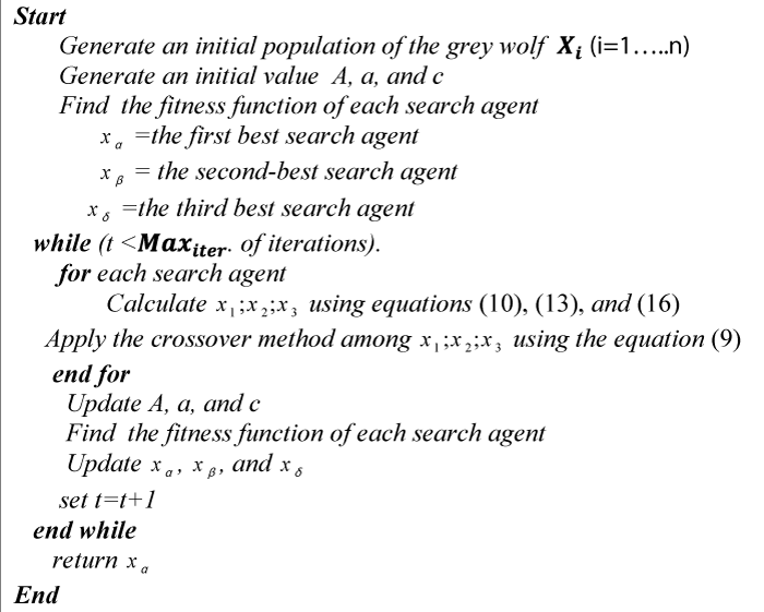
BGWO algorithm is displayed in figure 2 [10]:


Download Image

Figure 2: The pseudo code of the BGWO algorithm.

Naïve bayes classifier

Naïve Bayes is one of the great models used in the classifications, which calculates the probability that a particular feature belongs to a particular category it is assumed that the constituent features of the search space are restricted and dependent on certain conditions [10]. Naïve Bayes performs mostly well in terms of simplicity of construction and ease of implementation. From the example that describes the feature vector which is (X1, x2, …,xn), we will look for the class G which increases the probability of:

P ( X G )=P( x 1 , x 2 ,, x n |g)     (20) MathType@MTEF@5@5@+=feaaguart1ev2aaatCvAUfeBSjuyZL2yd9gzLbvyNv2CaerbuLwBLnhiov2DGi1BTfMBaeXatLxBI9gBaerbd9wDYLwzYbItLDharqqtubsr4rNCHbGeaGqk0Jf9crFfpeea0xh9v8qiW7rqqrFfpeea0xe9Lq=Jc9vqaqpepm0xbba9pwe9Q8fs0=yqaqpepae9pg0FirpepeKkFr0xfr=xfr=xb9adbaqaaeGaciGaaiaabeqaamaabaabaaGcbaaeaaaaaaaaa8qacaWGqbGaaiiOamaabmaapaqaa8qadaWcaaWdaeaapeGaamiwaaWdaeaapeGaam4raaaaaiaawIcacaGLPaaacqGH9aqpcaWGqbGaaeikaiaadIhapaWaaSbaaSqaa8qacaaIXaaapaqabaGcpeGaaiilaiaadIhapaWaaSbaaSqaa8qacaaIYaaapaqabaGcpeGaaiilaiabgAci8kaacYcacaWG4bWdamaaBaaaleaapeGaamOBaaWdaeqaaOWdbiaabYhacaWGNbGaaiykaiaabccacaqGGaGaaeiiaiaabccacaGGGcGaaiikaiaaikdacaaIWaGaaiykaaaa@53B5@

The Naïve Bayes method will allow conditional independence between the features in the data by expressing this probability P ( X G ) MathType@MTEF@5@5@+=feaaguart1ev2aaatCvAUfeBSjuyZL2yd9gzLbvyNv2CaerbuLwBLnhiov2DGi1BTfMBaeXatLxBI9gBaerbd9wDYLwzYbItLDharqqtubsr4rNCHbGeaGqk0Jf9crFfpeea0xh9v8qiW7rqqrFfpeea0xe9Lq=Jc9vqaqpepm0xbba9pwe9Q8fs0=yqaqpepae9pg0FirpepeKkFr0xfr=xfr=xb9adbaqaaeGaciGaaiaabeqaamaabaabaaGcbaaeaaaaaaaaa8qacaWGqbGaaiiOamaabmaapaqaa8qadaWcaaWdaeaapeGaamiwaaWdaeaapeGaam4raaaaaiaawIcacaGLPaaaaaa@3DBD@ as a result of those probabilities [11,12]:

P( X G )= π i=1 n P( X G )     (21) MathType@MTEF@5@5@+=feaaguart1ev2aaatCvAUfeBSjuyZL2yd9gzLbvyNv2CaerbuLwBLnhiov2DGi1BTfMBaeXatLxBI9gBaerbd9wDYLwzYbItLDharqqtubsr4rNCHbGeaGqk0Jf9crFfpeea0xh9v8qiW7rqqrFfpeea0xe9Lq=Jc9vqaqpepm0xbba9pwe9Q8fs0=yqaqpepae9pg0FirpepeKkFr0xfr=xfr=xb9adbaqaaeGaciGaaiaabeqaamaabaabaaGcbaaeaaaaaaaaa8qacaWGqbWaaeWaa8aabaWdbmaalaaapaqaa8qacaWGybaapaqaa8qacaWGhbaaaaGaayjkaiaawMcaaiabg2da9iabec8aW9aadaqhaaWcbaWdbiaadMgacqGH9aqpcaaIXaaapaqaa8qacaWGUbaaaOGaamiuamaabmaapaqaa8qadaWcaaWdaeaapeGaamiwaaWdaeaapeGaam4raaaaaiaawIcacaGLPaaacaGGGcGaaeiiaiaabccacaqGGaGaaeiiaiaacIcacaaIYaGaaGymaiaacMcaaaa@4E67@

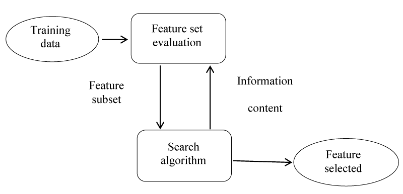
The feature selection method improves the performance of the algorithm by reducing the number of attributes used to describe a data set [6,13]. The purpose of features selecting in an algorithm is to reduce the number of genes used to improve classification and increase classification accuracy [14]. The feature identification algorithms consist of three parts:

1. Search algorithm: A subset of properties (features), which are part of the original features.

2. Fitness function: these input and digital assessment modes. The goal of the search algorithm is to draw attention to this function.

3. Classifier: It represents the required algorithm that uses the latest subset of genes (i.e., an algorithm that selects the most important features required) [15,16] (Figure 3).


Download Image

Figure 3: Filter control strategy.

One of the ways to select a feature on the predictive performance of a predefined algorithm is the wrapper method, which evaluates the quality and efficiency of certain features [17]. This is based on two-steps, based on a specific algorithm: (1) Searching for a subset of properties and features (2) Evaluate these specific features and attributes. In order to obtain learning performance or to reach some stop criteria we repeat (1) and (2) [12,18].

Mutual Information (MI)

Mutual information technology is widely used in feature selection and also in Sequence alignments. Mutual information technology arranges features according to their importance to data [12]. Mutual information technology is used to find out the relationship between some features and category classifications through the following relationship:

MutualInfo( X i ,C )= cC x i X i P( X i ,y)log P( X i ,y) P( X i )P(y)       (22) MathType@MTEF@5@5@+=feaaguart1ev2aaatCvAUfeBSjuyZL2yd9gzLbvyNv2CaerbuLwBLnhiov2DGi1BTfMBaeXatLxBI9gBaerbd9wDYLwzYbItLDharqqtubsr4rNCHbGeaGqk0Jf9crFfpeea0xh9v8qiW7rqqrFfpeea0xe9Lq=Jc9vqaqpepm0xbba9pwe9Q8fs0=yqaqpepae9pg0FirpepeKkFr0xfr=xfr=xb9adbaqaaeGaciGaaiaabeqaamaabaabaaGcbaaeaaaaaaaaa8qacaWGnbGaamyDaiaadshacaWG1bGaamyyaiaadYgacaWGjbGaamOBaiaadAgacaWGVbWaaeWaa8aabaWdbiaadIfapaWaaSbaaSqaa8qacaWGPbaapaqabaGcpeGaaiilaiaadoeaaiaawIcacaGLPaaacqGH9aqpdaGfqbqabSWdaeaapeGaam4yaiabgIGiolaadoeaaeqan8aabaWdbiabggHiLdaakmaawafabeWcpaqaa8qacaWG4bWdamaaBaaameaapeGaamyAaaWdaeqaaSWdbiabgIGiolaadIfapaWaaSbaaWqaa8qacaWGPbaapaqabaaal8qabeqdpaqaa8qacqGHris5aaGccaWGqbGaaiikaiaadIfapaWaaSbaaSqaa8qacaWGPbaapaqabaGcpeGaaiilaiaadMhacaGGPaGaciiBaiaac+gacaGGNbWaaSaaa8aabaWdbiaadcfacaGGOaGaamiwa8aadaWgaaWcbaWdbiaadMgaa8aabeaak8qacaGGSaGaamyEaiaacMcaa8aabaWdbiaadcfacaGGOaGaamiwa8aadaWgaaWcbaWdbiaadMgaa8aabeaak8qacaGGPaGaamiuaiaacIcacaWG5bGaaiykaaaacaGGGcGaaeiiaiaabccacaqGGaGaaeiiaiaabccacaGGOaGaaGOmaiaaikdacaGGPaaaaa@7411@

Where C is the set of categories, and Xi is the set of features in position i.

In mutual information technology, if there is a close correlation between the category and the feature, then the values of the mutual information will be large, but in the absence of a correlation between the feature and the category, the mutual information = 0. The mutual information can also be described as the degree of uncertainty in a feature that has been removed by knowing its category:

MutualInfo( X i ,C )=H( X i )H( X i \C )     (23) MathType@MTEF@5@5@+=feaaguart1ev2aaatCvAUfeBSjuyZL2yd9gzLbvyNv2CaerbuLwBLnhiov2DGi1BTfMBaeXatLxBI9gBaerbd9wDYLwzYbItLDharqqtubsr4rNCHbGeaGqk0Jf9crFfpeea0xh9v8qiW7rqqrFfpeea0xe9Lq=Jc9vqaqpepm0xbba9pwe9Q8fs0=yqaqpepae9pg0FirpepeKkFr0xfr=xfr=xb9adbaqaaeGaciGaaiaabeqaamaabaabaaGcbaaeaaaaaaaaa8qacaqGnbGaaeyDaiaabshacaqG1bGaaeyyaiaabYgacaqGjbGaaeOBaiaabAgacaqGVbWaaeWaa8aabaWdbiaabIfapaWaaSbaaSqaa8qacaqGPbaapaqabaGcpeGaaiilaiaaboeaaiaawIcacaGLPaaacqGH9aqpcaqGibWaaeWaa8aabaWdbiaabIfapaWaaSbaaSqaa8qacaqGPbaapaqabaaak8qacaGLOaGaayzkaaGaeyOeI0Iaaeisamaabmaapaqaa8qacaqGybWdamaaBaaaleaapeGaaeyAaaWdaeqaaOWdbiaacYfacaqGdbaacaGLOaGaayzkaaGaaiiOaiaabccacaqGGaGaaeiiaiaabccacaGGOaGaaGOmaiaaiodacaGGPaaaaa@5A17@

Where H(Xi) is an entropy in Xi and H(Xi\C) is an Xi entropy after knowing C so if knowledge of C provides a lot of information then H(Xi\C) will be low and therefore MutualInfo will be high. One disadvantage of the information exchanged favors rare features if the conditional probabilities are equal to P(Xi,y) and this may not always be the desired result [19].

The proposed algorithm

The proposed method for FMI _BGWO is two basic stages. In the first stage, the fuzzy mutual information (FMI) method is used to determine the most important feature based on a fuzzy Mam dani model created by relying on two input variables that represent the size of the sample data and the number of genes per sample. Three linguistic variables (high, mean and low) were selected for both input and output. The output range was also fixed between (10-50) to select the number of genes arranged by the MI method and which will be submitted to the second phase. In the second stage, the BGWO algorithm is used to reduce and define a certain number of features, which came from the first stage. In the BGWO method, the fitness function (FF) is used to evaluate wolves’ positions as follows:

FF=0.1*C+0.9*( q pq )     (24) MathType@MTEF@5@5@+=feaaguart1ev2aaatCvAUfeBSjuyZL2yd9gzLbvyNv2CaerbuLwBLnhiov2DGi1BTfMBaeXatLxBI9gBaerbd9wDYLwzYbItLDharqqtubsr4rNCHbGeaGqk0Jf9crFfpeea0xh9v8qiW7rqqrFfpeea0xe9Lq=Jc9vqaqpepm0xbba9pwe9Q8fs0=yqaqpepae9pg0FirpepeKkFr0xfr=xfr=xb9adbaqaaeGaciGaaiaabeqaamaabaabaaGcbaaeaaaaaaaaa8qacaWGgbGaamOraiabg2da9iaaicdacaGGUaGaaGymaiaacQcacaWGdbGaey4kaSIaaGimaiaac6cacaaI5aGaaiOkamaabmaapaqaa8qadaWcaaWdaeaapeGaamyCaaWdaeaapeGaamiCaiabgkHiTiaadghaaaaacaGLOaGaayzkaaGaaiiOaiaabccacaqGGaGaaeiiaiaabccacaGGOaGaaGOmaiaaisdacaGGPaaaaa@4E64@

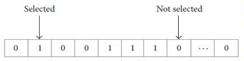
Where (q) is the length of the selected gene subset, (p) is the total number of features, (c) is the accuracy of the classification model. The vector in figure 2 consists of a series of binary values 0 and 1 that represents a subset of features, in this vector, all features can be selected.

The second stage of the proposed algorithm FMI_BGWO concentrates on the BGWO, specifically the wrapper in feature selection (Figure 4).


Download Image

Figure 4: A sample of the gene subset solution.

Through the method (FMI) obtained the most important features, these features will be entered in the algorithm (BGWO) to reduce them as a second stage. Using an algorithm (BGWO), a certain number of features are arranged and selected in the final classification process using the Naive Bayes classifier. Figure 5 presents an elaborate flowchart of the proposed FMI_BGWO structure.
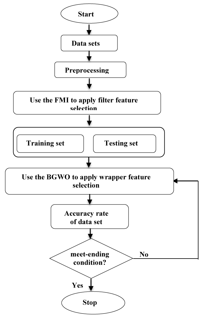

Download Image

Figure 5: The architecture of the proposed FMI_BGWO algorithm.

Algorithm 1: The proposed, FMI_BGWO, algorithm.
1: Set the initial parameters: Xi, A, a ,C , Max_iteration.
2: Apply the FMI filter method to determine a subset of features by importance.
3: Set the initial positions Eq. (2)

4: Evaluate dataset by fitness function and set X (t+1 MathType@MTEF@5@5@+=feaaguart1ev2aaatCvAUfeBSjuyZL2yd9gzLbvyNv2CaerbuLwBLnhiov2DGi1BTfMBaeXatLxBI9gBaerbd9wDYLwzYbItLDharqqtubsr4rNCHbGeaGqk0Jf9crFfpeea0xh9v8qiW7rqqrFfpeea0xe9Lq=Jc9vqaqpepm0xbba9pwe9Q8fs0=yqaqpepae9pg0FirpepeKkFr0xfr=xfr=xb9adbaqaaeGaciGaaiaabeqaamaabaabaaGcbaWaaCbiaeaaqaaaaaaaaaWdbiaadIfaaSWdaeqabaWdbiabgkziUcaakiaacIcacaWG0bGaey4kaSIaaGymaaaa@3EA3@ .
5: Set iteration i from 1 to Max_iteration.
6: Update gray wolf position and the parameter  Eq. (5) and Eq. (8).
7: When i ≤ Max_iteration stop satisfied and return get the best global solution.
8: Choosing a subset of the features identified by the BGWO algorithm.
9: Return the good of features (selected features).

The proposed algorithm FMI_BGWO is evaluated, and its interest is compared with the other competitor algorithms.

Datasets

We have selected (3) different classification problems from the literature to verify the effectiveness of the proposed algorithm for classification problems. From a repository UCI, a data set was obtained [20].

The target variable is a binary variable that includes a set of data where the binary variable represents the condition of the sick person who has good = 1 and bad = 0.

The following table shows the overall description of the data set (Table 1).

Table 1: Description of the used datasets.
Dataset # Samples # Features Target class
Leukemia 67 7130 2
Breast 168 2906 2

To correctly evaluate the proposed algorithm FMI-BGWO, the results were compared with the BGWO algorithm for feature selection.

The training and testing dataset for the proposed algorithm, FMI-BGWO, achieved the best results for the classification. For instance, in the breast dataset, the CA of the testing dataset is 82% by the FMI-BGWO which is higher than 100% by BGWO.

When comparing the BGWO algorithm with the proposed algorithm FMI-BGWO we note that the proposed algorithm FMI-BGWO has a clear advantage in terms of accuracy and classification capacity and BGWO worse than FMI-BGWO through the two datasets (Table 2).

Table 2: Classification performance on average of the algorithms used over 20 partitions (where the number in parentheses is the standard error).
Datasets Methods Number of
all features
Training dataset       Testing dataset
      CA SE SP MCC CA
Leukemia FMI-BGWO 21
(2.5386)
1
(0)
1
(0)
1
(0)
1
(0)
1
(0)
  BGWO 3550.9
(1.1511)
1
(0)
1
(0)
1
(0)
1
(0)
1
(0)
 
Breast FMI-BGWO 17.5
(1.9003)
1
(0) 
1
(0)
1
(0)
1
(0)
1
(0)
  BGWO 1447.5
(0.0412)
0.8286
(0.0366)
0.7646
(0.0486)
0.8563
(0.0352)
0.6072
(0.0822)
0.8839
(0.0478)

In this paper, to improve the performance of the classification of the big dataset, the FMI_BGWO method has been proposed. After the feature selection process, datasets were sent to Naïve Bayes. The results of the FMI_BGWO method were compared with the results of BGWO in table 2. Experimental results with a data set indicate that the proposed algorithm FMI_BGWO has a better classification accuracy and a number of features less than BGWO.

  1. Estévez PA, Tesmer M, Perez CA, Zurada JM. Normalized mutual information feature selection. IEEE Trans. 2009; 20: 189–201.
  2. Mirjalili S, Mirjalili SM, Lewis A. Grey wolf optimizer. Adv Eng Softw. 2014; 69: 46–61.
  3. Emary E, Zawbaa HM, Hassanien AE. Binary grey wolf optimization approaches for feature selection. Neurocomputing. 2016; 172: 371–381.
  4. Al-thanoon NA, Saber O, Yahya Z. Tuning parameter estimation in SCAD-support vector machine using firefly algorithm with application in gene selection and cancer classification. Comput Biol Med. 2018; 103: 262–268. PubMed: https://www.ncbi.nlm.nih.gov/pubmed/30399534
  5. Zaffar M, Iskander S, Hashmani MA. A study of feature selection algorithms for predicting students academic performance. Int J Adv Comput Sci Appl. 2018; 9: 541–549.
  6. Al-thanoon NA, Qasim OS, Algamal ZY. Selection of Tuning Parameter in L1-Support Vector Machine via. Particle Swarm Optimization Method. 2020; 15: 310–318.
  7. Singh N, Hachimi H. A new hybrid whale optimizer algorithm with mean strategy of grey wolf optimizer for global optimization. Math Comput Appl. 2018; 23: 14.
  8. Madadi A, Motlagh MM. Optimal control of DC motor using grey wolf optimizer algorithm. Tech J Eng Appl Sci. 2014; 4: 373–379.
  9. Emary E, Zawbaa HM, Grosan C. Experienced gray wolf optimization through reinforcement learning and neural networks. IEEE Trans Neural Netw Learn Syst. 2017; 29: 681–694. PubMed: https://www.ncbi.nlm.nih.gov/pubmed/28092578
  10. Manikandan SP, Manimegalai R, Hariharan M. Gene Selection from microarray data using binary grey wolf algorithm for classifying acute leukemia. Curr Signal Transduct Ther. 2016; 11: 76–83.
  11. Liu B, Blasch E, Chen Y, Shen D, Chen G. Scalable sentiment classification for big data analysis using naive bayes classifier. IEEE International Conference. 2013; 99–104.
  12. Chen J, Huang H, Tian S, Qu Y. Feature selection for text classification with Naïve Bayes. Expert Syst Appl. 2009; 36: 5432–5435.
  13. Ghamisi P, Benediktsson JA. Feature selection based on hybridization of genetic algorithm and particle swarm optimization. IEEE Geosci Remote Sens Lett. 2014; 12: 309–313.
  14. Alhafedh MAA, Qasim OS. Two-Stage Gene Selection in Microarray Dataset Using Fuzzy Mutual Information and Binary Particle Swarm Optimization. Indian J Forensic Med Toxicol. 2019; 13: 1162–1171.
  15. Karegowda AG, Jayaram MA, Manjunath AS. Feature subset selection problem using wrapper approach in supervised learning. Int J Comput Appl. 2010; 1: 13–17.
  16. Chuang LY, Chang HW, Tu CJ, Yang CH. Improved binary PSO for feature selection using gene expression data. Comput Biol Chem. 2008; 32: 29–38.
  17. Al-thanoon NA, Saber O, Yahya Z. Chemometrics and Intelligent Laboratory Systems A new hybrid fi re fl y algorithm and particle swarm optimization for tuning parameter estimation in penalized support vector machine with application in chemometrics. Chemom Intell Lab Syst. 2019; 184: 142–152.
  18. Zhao M, Fu C, Ji L, Tang K, Zhou M. Feature selection and parameter optimization for support vector machines: A new approach based on genetic algorithm with feature chromosomes. Expert Syst Appl. 2011; 38: 5197–5204.
  19. Zhang JR, Zhang J, Lok TM, Lyu MR. A hybrid particle swarm optimization–back-propagation algorithm for feedforward neural network training. Appl Math Comput. 2007; 185: 1026–1037.
  20. Blake CL, Merz CJ. UCI repository of machine learning databases. University of California, Department of Information and Computer Science, Irvine, CA. 1998