
More Information
Submitted: 18 December 2019 | Approved: 29 January 2020 | Published: 30 January 2020
How to cite this article: Yonis AL-Taie FA, Qasim OS. Classification of diseases using a hybrid fuzzy mutual information technique with binary bat algorithm. Ann Proteom Bioinform. 2020; 4: 001-005.
DOI: 10.29328/journal.apb.1001009
Copyright License: © 2020 AL-Taie FAY, et al. This is an open access article distributed under the Creative Commons Attribution License, which permits unrestricted use, distribution, and reproduction in any medium, provided the original work is properly cited.
Keywords: Classification; Binary Bat Algorithm (BBA); Mutual information; Fuzzy; Bigdata

Classification of diseases using a hybrid fuzzy mutual information technique with binary bat algorithm
Firas Ahmed Yonis AL-Taie* and Omar Saber Qasim
Department of Mathematics, University of Mosul, Mosul, Iraq
*Address for Correspondence: Firas Ahmed Yonis AL-Taie, Department of Mathematics, University of Mosul, Mosul, Iraq, Email: [email protected]; [email protected]
Genetic datasets have a large number of features that may significantly affect the disease classification process, especially datasets related to cancer diseases. Evolutionary algorithms (EA) are used to find the fastest and best way to perform these calculations, such as the bat algorithm (BA) by reducing the dimensions of the search area after changing it from continuous to discrete. In this paper, a method of gene selection was proposed two sequent stages: in the first stage, the fuzzy mutual information (FMI) method is used to choose the most important genes selected through a fuzzy model that was built based on the dataset size. In the second stage, the BBA is used to reduce and determine a fixed number of genes affecting the process of classification, which came from the first stage. The proposed algorithm, FMI_BBA, describes efficiency, by obtaining a higher classification accuracy and a few numbers of selected genes compared to other algorithms.
When dealing with bigdata, we strive to reduce the size of this data through the use of modern techniques, the most important of which is the feature selection process. In previous years, several algorithms have been proposed that simulate the behavior of some organisms in the search for food and the method they use in the research method [1]. Working on using them as a mathematical model to solve some complex problems. Kennedy and Eberhard proposed a binary version of the known Optimization of a Swarm Particle (PSO) called BPSO, where the conventional PSO algorithm was modified in order to address binary optimization problems [2,3] Rashedi, et al. proposed a binary version of the Gravitational Search Algorithm (GSA) called (BGSA) for feature selection [4] and Ramos, et al. presented their version of the Harmony Search (HS) for the same purpose in the context of theft detection in power distribution systems. This paper is divided into two stages of work, where the first stage begins using fuzzy in order to determine the features that affect the work results and then use the MI mutual information technology that enters only important data in the research process [5]. The second stage is to use the BBA binary bat algorithm [6].
Bat algorithm
Bats are the only mammals that have wings and have enormous capabilities and efficiency to make them be of interest to researchers from these features is their ability to echolocation this feature can be considered a kind of natural sonar [7]. Bats work to produce sound pulses of different frequencies and very fast, and then wait for these pulses to return to them after they collide with prey, and then calculate the distance between it and prey depending on the frequency of the sound waves and the time period Back and forth [8]. In this way, bats consider among the creatures that are able to devour themselves at night and in the dark darkness, they have bats that are able to distinguish between moving and fixed targets and know the direction of movement of these targets, this process is done in a small part of the time [8]. The author of this algorithm YANG considers the behavior of the bat to be an ideal method of selection and path improvement [1] (Figure 1). He then developed them to resemble a group of bats looking for food/prey using echo-positioning [9,10]. Some improvement rules have been developed as follows:
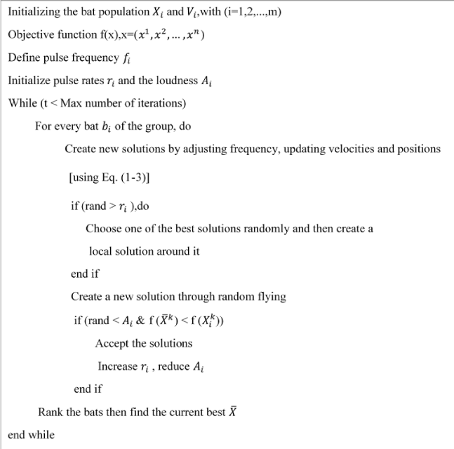
Figure 1: Pseudo code of bat algorithm.
1. All bats have echo position property to estimate distance and also know the difference between (obstacles and prey) in an amazing way.
2. Bats fly in randomly velocity (Vi) and position (Xi) with constant frequency fmin changing in wavelength (λ) and sound loudness (Ao), bats have the ability to adjust wavelength or pulses frequency produced from it and is able to adjust the rate of pulse r ϵ [0,1] According to the prey dimension.
3. The loudness of bats can vary in many ways, but YANG assumes that the loudness can change within a given curve from a large positive value Ao to a minimum value Amin and be constant. The default movement of the bat is given by updating the position and updating the velocity using the following mathematical model:
Where represents the velocity of the new bat.
Where represents the new position, represents the best current global solution for a site that can be considered the best for the decision variable.
Where f1 the frequency for each bat is bi, β is a random number whose value is between [0,1].
YANG introduced the idea of using random paths technique to improve the apparent contrast in possible solutions by selecting one of the current best solutions and then using it to create a new solution for all bats in the group as [11]:
Where ϵ is a random number and has a value of [-1,1], is the average of all sounds coming from all bats in this step. The technique is balanced by adjusting the loudness and pulse emission rate as follows:
α and y are constants, of the algorithm and in the first steps the emission rate and loudness are chosen randomly and within the period ϵ [0,1] and ϵ [0,1].from the previous equations, it will be noted that bats follow the frequency change, which works to accelerate their access to the best solution [6] .
In order to solve problems in discrete space, the copy of the bat algorithm has been updated to a binary version that deals with problems on a vector basis [0,1] where molecules can travel to all corners of any excessive material using only 0 or 1 values [12]. This means that the bat algorithm (BBA) is somewhat similar to the basic algorithm (BA), but depending on the search space where the BA operates at continuous distances while BBA search is based on the discrete space by 0 and 1 this process requires a function that changes values between 0 and 1 and is called the transfer function [13]. The process of choosing this function depends on certain conditions in which it must be met:
1. The scope of this function must be related to the range [0,1], as it represents the probability of a particle changing its position.
2. The transfer function should provide the greatest possible change of position to change the absolute velocity value. Some particles with a great absolute value of their velocity can be moved away from the optimal solution and therefore must be switch repositioned in the following iterations.
3. The previous phrase applies for the smallest probability to change position even if the absolute velocity was too small.
In this paper, we rely on the (sigmoid function) as a transport function by which the locations of all molecules are converted to binary values:
According to this function can be replaced Eq. (2) with Eq. (8):
Where (Normal distribution).
The last equation is a mechanism for giving binary values to any bat from a swarm the bats in space.
Mutual Information (MI)
We often find a lot of information for random coherent and related variables, and the degree of correlation of these variables and their effect on some of them can be inferred through the Mutual information [14].
Where H be the entropy of the discrete random variable X conditioned on the discrete random variable Y taking a certain value. That means the information about y that we got and is meant to be Mutual information I (X;Y).
Otherwise, I (X;Y) = 0, if X and Y are completely unrelated.
The information Mutual was mainly applied to filter feature settings to measure the correlation between specific features and some class classifications [15]. There is a classical implementation of the mutual information method in several of the feature classification metrics [16] (Figure 2). One of the most important applications of this theory is to choose the feature as it will evaluate the importance of the features and arrange them according to their importance, in other words this theory will arrange the features in ascending order according to the impact of each feature on the final results of the data and thus will reduce the number of features included in the calculations, which accelerates the work of the program [17]. In the following relationship, it will be indicated by a wide range of features and classifications:
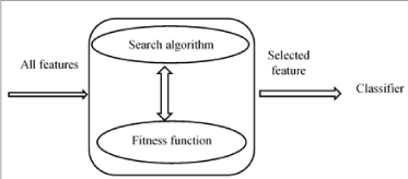
Figure 2: The strategy of filter control.
The process of inferring information exchanged between specific features, the process goes easily, but the difficulty lies when evaluating a full set of features and finding the link of each feature with a series of other features. Each feature may not give a complete picture of the situation, but the addition process between them can clarify that image [18,19]. Between N variables (X1, X2 …XN) and the variable (Y), the chain rule is:
It is possible to specify the exchanged information as a type of measure to reduce uncertainty about classification labels, where the "fitness function" maximizes the values of information exchanged [3,20].
Features selection
The feature selection method reduces the number of features used to describe a set of big datasets in order to improve the performance of the algorithm. The aim of this method is to reduce the number of features used and reduce the time required to obtain results, which leads to an increase in the accuracy of classification [18,21] (Figure 3). The feature selection algorithm can be represented in three stages:
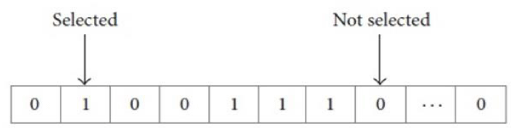
Figure 3: A sample of the feature selection subset solution.
1. Search algorithm: it evaluates the total number of features entered and selects the important part from it.
2. Fitness function: it transfers data to the binary system to select features that correspond to the number 1.
3. Classifier: it analyzes the input data that came out of the fitness function to give more accurate results.
Propose algorithm
The proposed method FMI_BBA consists of two basic stages. In the first stage, the fuzzy mutual information (FMI) method is used to determine the most important features by fuzzy Mamdani model that was created on the basis of two variables of the inputs that represent the size of the data and the number of features for each type of this data. Three variables were selected for each of the inputs and outputs on a picture (low, medium, high), then a range for these outputs is determined between (10 - 50) in order to determine the number of features that will enter the MI technique that will, in turn, be sent to the second stage the second stage, The BBA algorithm is used to reduce and specify a certain number of features, which came from the first stage by randomly synchronizing the vector [0,1] where the features corresponding to value 1 enter the classification function and neglect the features that correspond to the value 0.
Where C the accuracy of the classification model is, q is length of selected feature, p is the total number of features.
The second phase of the proposed algorithm FMI_BBA focuses on the BBA, specifically the wrapper in feature selection. After obtaining the most important features through the FMI method, these features are introduced into the BBA algorithm to be reduced as a second stage (Algorithm 1). A specific number of features arranged using the BBA algorithm are adopted and selected in the final classification operation using the Naive Bayes classifier. (Figure 4) presents a detailed flowchart of the proposed FMI_BBA framework.
| Algorithm 1: The proposed FMI_ BBA, algorithm |
| 1: Set the initial parameters: r, n, cc1, dd1, Max_iteration, 2 : Apply MI filter technique to select a subset of features depending on their importance |
| 3: Set the initial velocities and positions using, Eq. (1) and Eq. (2) |
| 4: Evaluate dataset by fitness function and set . |
| 5: Set iteration i from 1 to Max_iteration. |
| 6: Update data velocity and position according to Eq. (1) and Eq. (2). |
| 7: When I ≤ Max_iteration stop satisfied and return get the best global solution. 8: Choosing the subset from the features specific by the BBA algorithm. |
| 9: Return the good of features (selected features). |
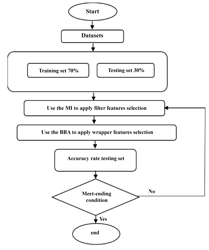
Figure 4: The architecture of the proposed FMI_BBA algorithm.
Experimental results
The suggested algorithm FMI_BBA is evaluated and compared with other evolutionary algorithm.
Datasets
The application of the proposed algorithm to a group of bigdata is one way to verify its efficiency in solving classification problems. Table 1 is illustrated applying the algorithm to some data obtained from the UCI repository [22].
| Table 1: Description of the data sets used. | |||
| Dataset | # Samples | # Features | Target class |
| Ovarian | 253 | 15155 | 2 |
| Dlbcl | 77 | 7130 | 2 |
Evaluation criteria
Classification efficiency is measured by quality (SP), matthew correlation coefficient (MCC), classification accuracy (AC) and sensitivity (SE) these metrics are defined by the following:
Where TP, TN, FP, and FN be the numbers of true positive, true negative, a false positive and false negative of the confusion matrix, respectively, where the values of these criteria represent the strength of the classification process and the proportionality between them is direct.
Discussion and analysis
The algorithm proposed in this paper is compared with both the binary genetic algorithm (BGA) and the (BBA) original algorithm.
The data set is divided into 30% as a test group in our experiments and the rest is used as training data. A 20-fold is set to obtain the best reliable ratingt table 2, the evaluation criteria are compared with some other evolutionary algorithms. It shows that fewer than the total number of features have been selected and the accuracy of the proposed algorithm classification compared to other classification algorithms.
Table 2 shows that the data for both the training group and the test group achieved the best results classification. For example, in the leukemia dataset, the accuracy (AC) of the data for the train group represented 97% in the proposed algorithm FMI_BBA and 90% in BBA. And 92% in BGA.
| Table 2: Classification of the performance of algorithms on average of more than 20 sections (the number in parentheses represents the standard error). | |||||||
| Datasets | Methods | Training dataset | Testing dataset | ||||
| Ovarian | FMI-BBA | 18.2 (0.3071) | 0.9768 (0.0591) |
0.9965 (0.0195) |
0.9559 (0.0455) |
0.9725 (0.0257) |
0.9044 (0.0958) |
| BBA | 483.15 (0.3170) |
0.6610 (0.0383) |
0.6105 (0.0507) |
0.8062 (0.0368) |
0.3643 (0.0552) |
0.7544 (0.0891) |
|
| BGA | 399.2500 (0.3230) |
0.8880 (0.0871) |
0.9533 (0.1310) |
0.8458 (0.1240) |
0.9627 (0.1654) |
0.9299 (0.0364) |
|
| Dlbcl | FMI-BBA | 14.2 (0.2608) | 0.9721 (0.0358) |
0.9256 (0.0745) |
0.91769 (0.0812) |
0.9346 (0.0419) |
0.9711 (0.0824) |
| BBA | 474 (0.2721) |
0.9048 (0.0416) |
0.9148 (0.0547) |
0.8880 (0.1030) |
0.7205 (0.1284) |
0.9640 (0.0448) |
|
| BGA | 383.55 (0.3021) |
0.9548 (0.248) |
0.9658 (0.0258) |
0.9320 (0.0403) |
0.8992 (0.0541) |
0.9366 (0.0096) |
|
This research has proposed a BBA algorithm with FMI to evolve the classification performance by depending on a subset of the dataset. A Naïve Bayes classifier was used to classify the dataset obtained from all algorithms. Results obtained from the FMI-BBA are compared with BPSO and BGA in table 2. Experimental results with the four datasets suggest that the proposed algorithm, FMI-BBA has a better classification achievement with a little selected gene.
- Yang XS. A new metaheuristic bat-inspired algorithm. Nat inspired Coop Strateg Optim. 2010; 65-74.
- Alhafedh MAA, Qasim OS. Two-Stage Gene Selection in Microarray Dataset Using Fuzzy Mutual Information and Binary Particle Swarm Optimization. Indian J Forensic Med Toxicol. 2019; 13: 1162-1171.
- Qasim OS, Algamal ZY. Feature selection using particle swarm optimization-based logistic regression model. Chemom Intell Lab Syst. 2018; 182. 41-46.
- Jadidi Z, Muthukkumarasamy V, Sithirasenan E, Sheikhan M. Flow-based anomaly detection using neural network optimized with GSA algorithm in 2013. IEEE 33rd International Conference on Distributed Computing Systems Workshops. 2013; 76-81.
- Chen W, Xu W. A Hybrid Multiobjective Bat Algorithm for Fuzzy Portfolio Optimization with Real-World Constraints. Int J Fuzzy Syst. 2019; 21: 291-307.
- Pourpanah F, Lim CP, Wang X, Tan CJ, Seera M, et al. A hybrid model of fuzzy min–max and brain storm optimization for feature selection and data classification. Neurocomputing. 2019; 333: 440-451.
- Guha D, Roy PK, Banerjee S. Binary t Algorithm Applied to Solve MISO-Type PID-SSSC-Based Load Frequency Control Problem. Iran J Sci Technol. 2019; 43: 323-342.
- Gupta D, Arora J, Agrawal U, Khanna A, de Albuquerque VHC. Optimized Binary Bat algorithm for classification of white blood cells. Measurement. 2019; 143: 180-190.
- Pebrianti D, Ann NQ, Bayuaji L, Abdullah NRH, Zain ZM, et al. Extended Bat Algorithm (EBA) as an Improved Searching Optimization Algorithm. Proceedings of the 10th National Technical Seminar on Underwater System Technology 2018. 2019; 229-237.
- Al-Azzawi SF. Stability and bifurcation of pan chaotic system by using Routh–Hurwitz and Gardan methods. Appl Math Comput. 2012; 219: 1144-1152.
- Jayabarathi T, Raghunathan T, Gandomi AH, The bat algorithm, variants and some practical engineering applications: a review. Nature-Inspired Algorithms and Applied Optimization. Springer. 2018; 313-330.
- Li G, Le C. Hybrid Binary Bat Algorithm with Cross-Entropy Method for Feature Selection. 4th International Conference on Control and Robotics Engineering (ICCRE). 2019; 165-169.
- Hong WC, Li MW, Geng J, Zhang Y. Novel chaotic bat algorithm for forecasting complex motion of floating platforms. Appl Math Model. 2019; 72: 425-443.
- Estévez PA, Tesmer M, Perez CA, Zurada JM. Normalized mutual information feature selection. IEEE Trans Neural Networks. 2009; 20: 189-201. PubMed: https://www.ncbi.nlm.nih.gov/pubmed/19150792
- Patel H, Shah M. Rough Set Feature Selection Using Bat Algorithm. 2016.
- Bennasar M, Hicks Y, Setchi R. Feature selection using joint mutual information maximization. Expert Syst Appl. 2015; 42: 8520-8532.
- Yang H, Moody J. Feature selection based on joint mutual information. Proceedings of international ICSC symposium on advances in intelligent data analysis. 1999; 22–25.
- Chen H. Distributed Text Feature Selection Based On Bat Algorithm Optimization. 10th IEEE International Conference on Intelligent Data Acquisition and Advanced Computing Systems: Technology and Applications (IDAACS). 2019; 1: 75-80.
- Entesar A, Saber O, Al-Hayani W. Hybridization of Genetic Algorithm with Homotopy Analysis Method for Solving Fractional Partial Differential Equations.
- Al-Thanoon NA, Qasim OS, Algamal ZY. A new hybrid firefly algorithm and particle swarm optimization for tuning parameter estimation in penalized support vector machine with application in chemometrics. Chemom Intell Lab Syst. 2019; 184: 142-152.
- Al-Thanoon NA, Qasim OS, Algamal ZY. Tuning parameter estimation in SCAD-support vector machine using firefly algorithm with application in gene selection and cancer classification. Comput Biol Med. 2018; 103: 262-268. PubMed: https://www.ncbi.nlm.nih.gov/pubmed/30399534
- Blake C, Merz CJ. UCI repository of machine learning databases, Department of Information and Computer Science. Univ California Irvine CA. 1998. 55.